Math
Sine and cosine
Trigonometry deals with calculations around triangles, much of which was already known in ancient times. We also make extensive use of various functions in computer graphics, and we will look at two very important ones, the sine and the cosine, in more detail.
If we want to draw a circle on a computer screen, it’s not as easy as it is on paper. On paper, all you need is a starting point and the radius with which to draw a circle by hand or with compasses.
On the computer, we don’t have compasses and instead we need to draw a number of points which then form a circle. For this we now use sine and cosine.
In the diagram below, we see a rectangular triangle where one opposite side of the right-angled corner has a length of 1. This side is called the hypotenuse. If the side has length one and we insert the angle a from 0 to 360 degrees, 360 triangles form. The points of the outer edge then form a circle with a radius of 1. This is the unit circle.
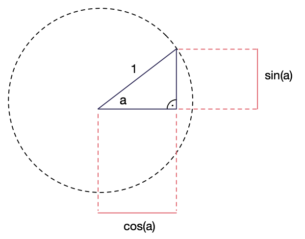
As we can see further, the horizontal side of the triangle has the length cos(a), i.e. the value cosine of the angle a corresponds to the length of the one of the two cathets called shorter sides of the triangle.
The second, vertical side has the length sine of a.
The sine and cosine values can also be looked up in tables if you don’t have a computer handy. For each angle we can find the corresponding value in such tables.
Now, it is interesting to note that cos(a) actually corresponds to our X coordinates, and the sin(a) corresponds to our Y coordinates. So if we have an angle, we can use these functions to work out the coordinate of the outer corner of the triangle.
Example:
const LENGTH = 100 # 20 ... 119
const DELAY = 100 # 20 ... 1000
const STEP = 0.1 # 0.1 ... 1.0

angle = 0.0

def onDraw():
    push()
    background(0,0,0)
    noFill()
    x = cos(angle)*LENGTH
    y = sin(angle)*LENGTH

    translate(120,120)
    stroke(200,200,200)
    drawCircle(0,0,LENGTH)

    stroke(0,0,150)
    drawTriangle(0,0,x,0,x,y)

    stroke(100,100,100)

    drawLine(0,0,x,y)
    drawCircle(0,0,2)
    stroke(200,0,0)
    drawCircle(x,y,2)

    update()
    delay(DELAY)
    pop()

    angle = angle + STEP
    if angle > PI * 2: angle = 0
This program draws the plane triangle discussed. After each pass, the angle is increased by 0.1. Note: the angle is in units of radians, not degrees.
To get a circle of any size from the unit circle with radius 1, we simply multiply by the desired length (LENGTH) on the following lines:
x = cos(angle)*LENGTH
y = sin(angle)*LENGTH
Degree/ radian measure
An angle can be expressed in degrees or radians.
If we consider a round pie and cut it into pieces, we can specify angles in two ways: In degree measure, the entire pie comprises 360 degrees. In radians, the maximum angle that corresponds to 360 degrees is “2 * PI”, which is approximately 6.2831 radians.
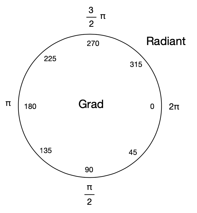
Example: a quarter of a pie has a 90 degree angle or angle 6.2831/4 ~ 1.57 in radians.
The values can be converted via built-in functions:
Degree from radian:
degree = deg(radiant)
Radian from degree:
radiant = rad(degree)
Vector
A (two-dimensional) vector is figuratively speaking an arrow with a direction and a length. In our Cartesian coordinate system, a vector is specified by means of two numbers x and y.
Vectors can be used to make various calculations, which are a great simplification in computer graphics and animation, among other things. For example, acceleration and velocities can be represented as vectors, whereby simple physical processes can be implemented.
In NanoPy there is also a vector class “vector”, which already contains ready vector calculation functions. The class knows the two variables x and y (data type: float).
Initializations:
v1:vector
declares a vector object with x=0, y=0
v2 = vector(x = 10, y = 20)
declares an object with x = 10, y = 20
v3:vector
v3.random()
v3.mulScalar(10)
Declares an arbitrary direction vector with a length of 10.
v4:vector
v4.fromAngle(PI/2)
v4.mulScalar(20)
Declares a direction vector with angle PI/2 radians and length 20 pixels.
See also Vector Functions.
Unit circle
The unit circle is the circle that has a radius of 1.
Calculating with variables
When one deals with programming, mathematical concepts also come up quickly. For example, we often calculate with variables that we also know in algebra. In addition, we have the basic arithmetic operations that you learn in school at our disposal. And, of course, many more possibilities.
We summarize the most important points:
As in algebra, you can use letters or even whole words in addition to numbers when doing calculations on a computer. We call these placeholders variables.
To calculate with variables, you simply write down a formula using letters or even words. Example:
To calculate the volume of a building, you need to know the length, width and height. So the volume is calculated like this: v = volume, b = width, h = height and l = length.
v=b*h*l
This formula is universal and since there are no numbers inserted, you can use the formula over and over again for different combinations of numbers.
In the example above, we used “=” to define something. We say v “is equal to” something and define a formula after the equal sign.
On the right side of the formula, we used multiplication “*”. As with calculators, we have different arithmetic operations that we can use:
| + | Addition |
| - | Subtraction |
| / | Division |
| * | Multiplication |
| % | Modulo |
Additionally, we can also negate a number by prepending “-“ or change the execution order by using the round brackets “(“ and “)”.
Here are some examples:
a = 10
b = 10 * a
c = b - a
d = c % 7
e = (a + b) * (c-d)
f = -e
a is assigned the value 10. b is 10 * a, i.e. 100. c is b - a, i.e. 100-10 = 90.
d is c % 5. The % drawing means that d is assigned the remainder value of the integer division by 5. I.e. c=90, 90 % 7 = 6, because 7 has only 12 times in 90 place (84) and then there remains a remainder of 6. For e, we first calculate (a +b) and (c- d) and only then multiply (110 * 84 = 9240). For f, we negate e, i.e., f becomes -9240.
Example 1:
w = 20

def onDraw():
    background(0,0,0)
    fill(255,255,255)
    drawRectangle(20,20,w,w*2)
    update()

def onClick():
    w = w + 10
    if w > 120: w = 20
    delay(100)
Using the function “drawRectangle(x,y,width, height)” we draw a rectangle. “x” and “y” correspond to the starting point, “width” to the width and “height” to the height. Instead of numbers, we specified “w” as the width and “w*2” as the height. When any button is clicked, “w” is incremented by 10 at a time, which causes a larger rectangle to appear the next time it is drawn. w is our variable, which we can use anywhere. This allows the program to draw different rectangles at the click of a button, depending on what w’s value is.
Example 2:
x = 0

def onDraw():
    ``if x == 0:
        background(0,0,0)
    x = x+1
    if x > 240:
        x=0
    y = x % 40
    drawLine(x,0,x,y)
    update()
In this example we are using modulo function. Have two variables. “x” is incremented from 0 to 240. “y” contains the formula “x % 40” and so assigns “y” the remainder of the division by 40. I.e. the number runs through a series from 0 to 39.